Placing the states
Placement is the part of the pipeline that decides where each state sits and how big it is. Everything downstream — carving states into district cells, matching those cells to real districts — happens inside shapes that have already stopped moving. See the index for all three.
Every figure below is generated by R/40_doc_figures.R from the build artefacts,
so it cannot drift from what the pipeline actually does. Re-run it after any
build and the pictures update.
There is also an interactive version you can step through, hosted alongside the maps themselves.
1. Start from the real map
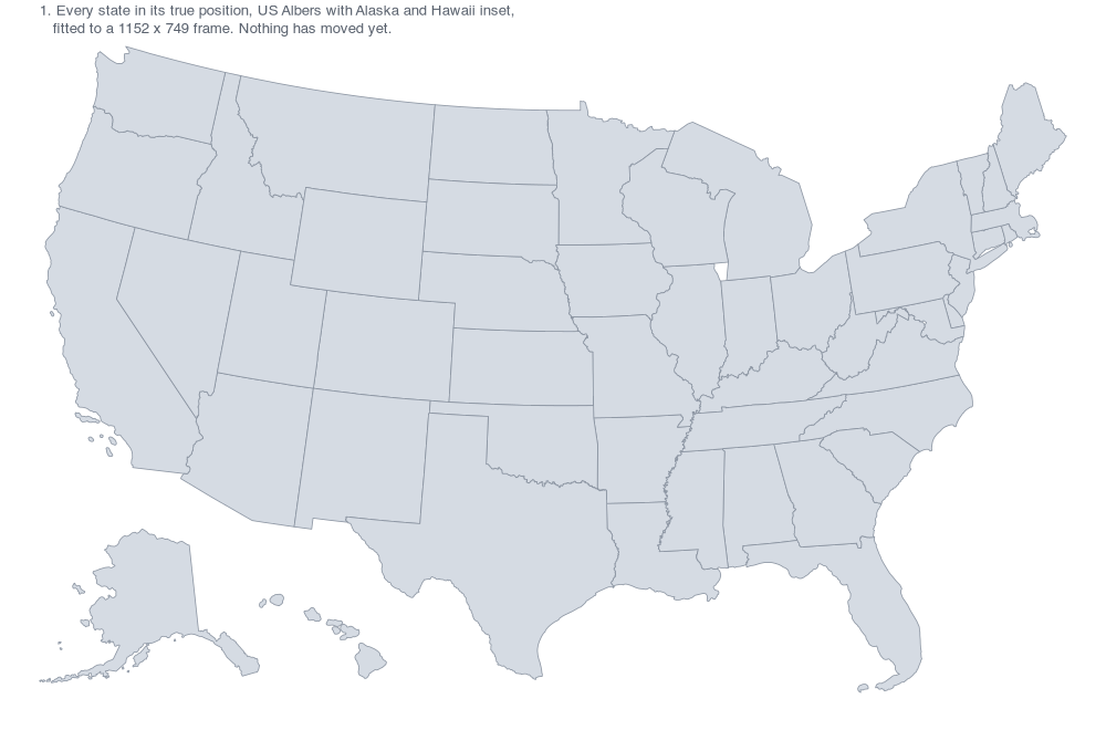
A US Albers projection with Alaska and Hawaii inset, fitted to a 1152 × 749 frame. Area here is land area, which is exactly the thing that misleads: Wyoming covers twelve times the ground of New Jersey and holds one seat against its twelve.
2. Resize each state to its seat count
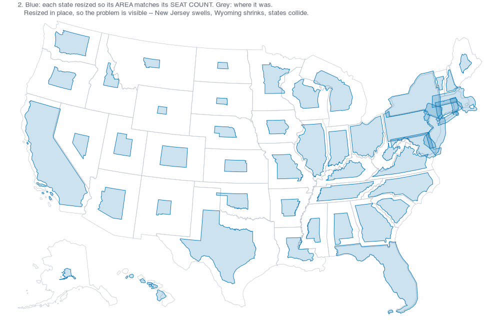
Scale each state so its area becomes proportional to its share of the 435 seats:
k = sqrt( totalArea × seatShare / area / AREA_DIVISOR )
New Jersey grows by 1.83×, Wyoming shrinks to 0.16×. The figure does this in place to show the problem it creates: the country now collides with itself, badly in the Northeast.
AREA_DIVISOR is a single global constant that sets how much of the frame the
cartogram fills. The notebook hard-codes 2.5; ours is 2.898, recovered from the
layout slots rather than guessed — see the README.
3. Bring in the slots
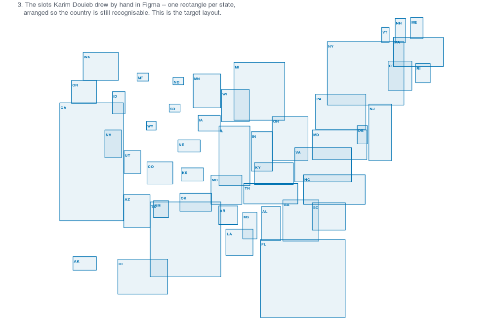
Karim Douieb drew one rectangle per state by hand in Figma, arranged so the
country stays recognisable. Nothing computes these — they are a designed object,
and sh/03_extract_layout.js lifts them straight out of his notebook into
R/statepos.R. They are the target each state aims for.
4. Move each state to its slot
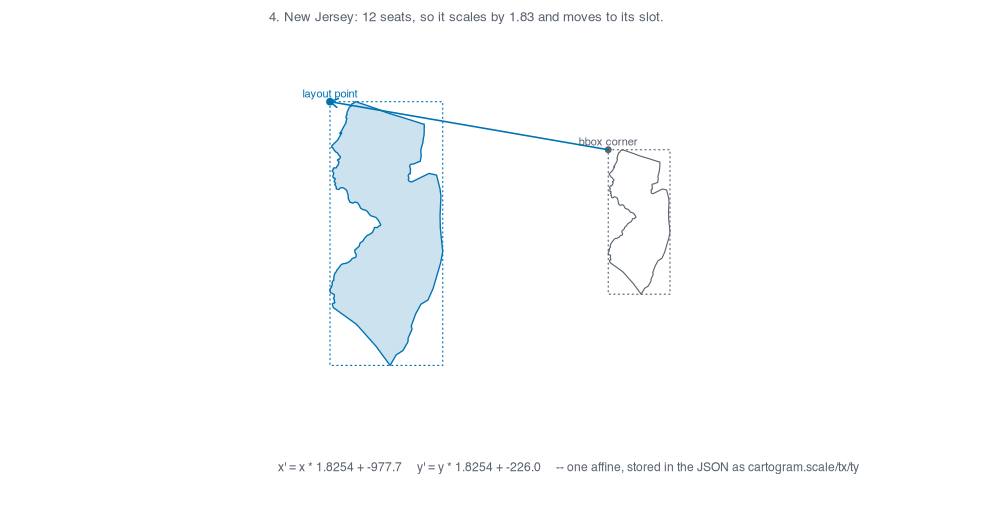
Scale about the state’s own bounding-box corner, then move that corner onto the slot’s corner. Those two operations collapse into a single affine:
x′ = x · k + tx y′ = y · k + ty
which is exactly what the output JSON stores per state as
cartogram.scale/tx/ty. No renderer has to re-derive it — the election viewer
and the apportionment viewer both just apply it.
5. Push apart until nothing touches
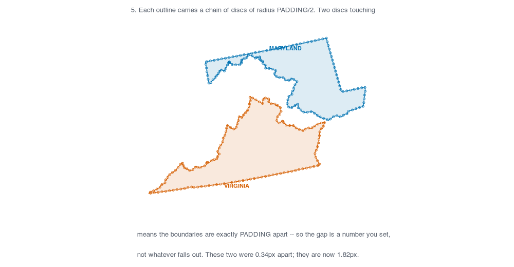
The slots were drawn for one particular set of sizes. A different apportionment gives different sizes, so states can still end up touching.
Each outline carries a chain of discs of radius PADDING/2. Two discs from
different states touching then means exactly one thing: their boundaries are
PADDING apart. Maryland and Virginia were 0.34 px apart — visually
touching — and are now 1.82 px.
Why discs, rather than the obvious alternatives? Measured over the same 1,225 state pairs:
| Collision test | Pairs flagged | States moved | Result |
|---|---|---|---|
One circle per state (d3.forceCollide) |
80 | — | Demands 117 px of separation. The country comes apart. |
| One box per state (rectangle cartogram) | 34 | 37 of 50 | Tennessee ends up between Kentucky and North Carolina. |
| The outlines themselves | 1 | 2–4 | Correct, but the gap is whatever falls out. |
| A chain of discs along each outline | 1 | 3–11 | Correct, and the gap is a number you set. |
California is why. It is a diagonal sliver whose bounding circle has a 148 px radius against a 155 px width, so a circle test believes it collides with half the West; its bounding box overlaps Nevada’s while the shapes come nowhere near each other.
The hand corrections
Three coarse adjustments in R/statepos_tweaks.R set the arrangement the disc
pass then refines. Each exists because the layout was drawn for one particular
set of state sizes, and each direction was found by measurement rather than
intuition — in two of the three the obvious direction made things worse.
| States | Offset | Why | Gap before → after |
|---|---|---|---|
| New England — ME, NH, VT, MA, RI, CT | (-4, -11) |
Connecticut sat over the eastern end of New York’s Long Island | 0 → 3.00 px |
| West Virginia | (+3, -6) |
Interlocks with Virginia; their shapes wrap around each other | 0 → 10.77 px |
| Louisiana | (+4, -3) |
Was touching Texas rather than overlapping it | 0.1 → 6.80 px |
Connecticut / New York. The one genuine overlap: 108 px² on the election map, 141 px² on the 2020–2030 projection. Moving Connecticut east — the obvious direction — makes it worse, because Long Island runs east underneath Connecticut’s slot. Up and to the left lifts it clear.
All six New England states move together. They read as one cluster, and the
spacing between them is part of what makes the region legible, so sliding
Connecticut out on its own would leave it detached from Rhode Island and
Massachusetts. relax_discs() knows about this too: groups makes New England a
single rigid body, so the solver can never break it apart either.
Virginia / West Virginia. These two interlock, and overlapped by ~17 px² whenever West Virginia held three seats. Lifting West Virginia clears it; the small rightward component widens the gap in the builds where West Virginia is largest.
Louisiana / Texas. Not really an overlap — 0.2 px² on the projection, with a 0.1 px gap. But two shapes that close read as colliding, which is what matters for a graphic. Moving Louisiana right and up opens a real gap without closing the one to Mississippi, which is now 4.36 px.
Set TWEAKS=0 to build without any of them.
6. Placement finished
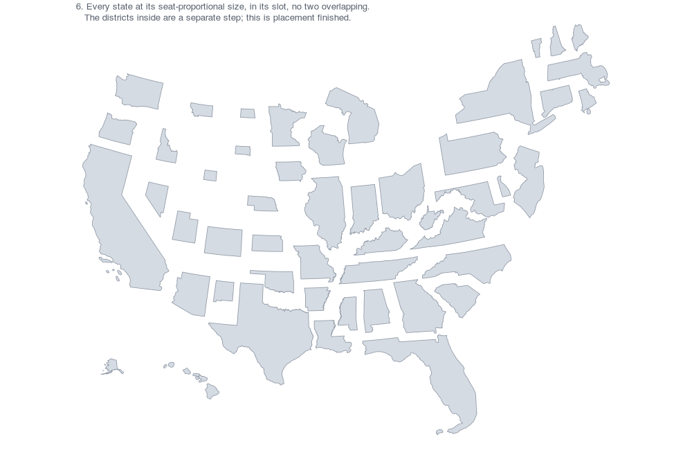
Every state at its seat-proportional size, in its slot, with no two overlapping.
Implementation notes
Rigid bodies. d3.forceCollide moves each node independently, which would
tear a state into hundreds of loose discs. Corrections translate every disc of a
state together, and groups makes New England a single body — the six states
read as a cluster, and sliding Connecticut out of it to satisfy a constraint
would be a worse outcome than the constraint.
Sequential projection, not summed forces. Accumulating each pair’s push and applying the sum stalls: Maryland is boxed in by Pennsylvania, Delaware and New Jersey, so its competing pushes cancel and it sits at an equilibrium with the Virginia constraint still violated. Applying each correction immediately — Gauss-Seidel — propagates the slack around the chain.
Deepest penetration, not the mean. Averaging hundreds of disc pairs along a shared edge dilutes the push, because normals on opposite sides of an interlocking boundary partly cancel.
An infeasible padding is worse than a smaller one. The solver oscillates against the spring and stops mid-swing. Asking for 3 px leaves 0.80 px between Connecticut and New York, where 2 px converges in three iterations and delivers 1.82 px. It warns when it fails to reach the target.
Seeded from the hand tweaks. R/statepos_tweaks.R sets the coarse
arrangement — New England shifted as a block, West Virginia lifted off Virginia,
Louisiana off Texas — and the disc pass enforces the gap on top. Seeding from the
raw layout does not work: on the 2020–2030 projection it thrashes for 400
iterations and leaves 123 px² of Connecticut still on Long Island.
Known limit. Only the boundary is sampled, so a state entirely inside another’s concave bay, touching nothing, would not register. That cannot happen in this layout.
Where the code lives
| File | Role |
|---|---|
R/10_build_cells.R |
Computes congressScale, calls the relaxation, writes lay_dx/lay_dy |
R/statepos.R |
The Figma layout, generated from the notebook — do not hand-edit |
R/statepos_tweaks.R |
Hand corrections, applied on top of the generated layout |
R/lib_discs.R |
Boundary-disc sampling and the rigid-body solver |
R/lib_relax.R |
The earlier polygon and bounding-box solvers, kept for comparison |
R/40_doc_figures.R |
Generates every figure on this page |
Switches: RELAX (discs default, or polygon / box / none), PADDING
(2 px), TWEAKS=0 to ignore the hand corrections.