Matching cells to districts

Carving a state produces the right number of equal-area cells, but nothing about which cell belongs to which district. Cell 7 is not district 7 — it is just the seventh polygon the algorithm happened to emit.

Something has to pair them, and the pairing matters: it is what the morph animates along, and what makes the transition read as districts moving rather than shapes dissolving into unrelated shapes.

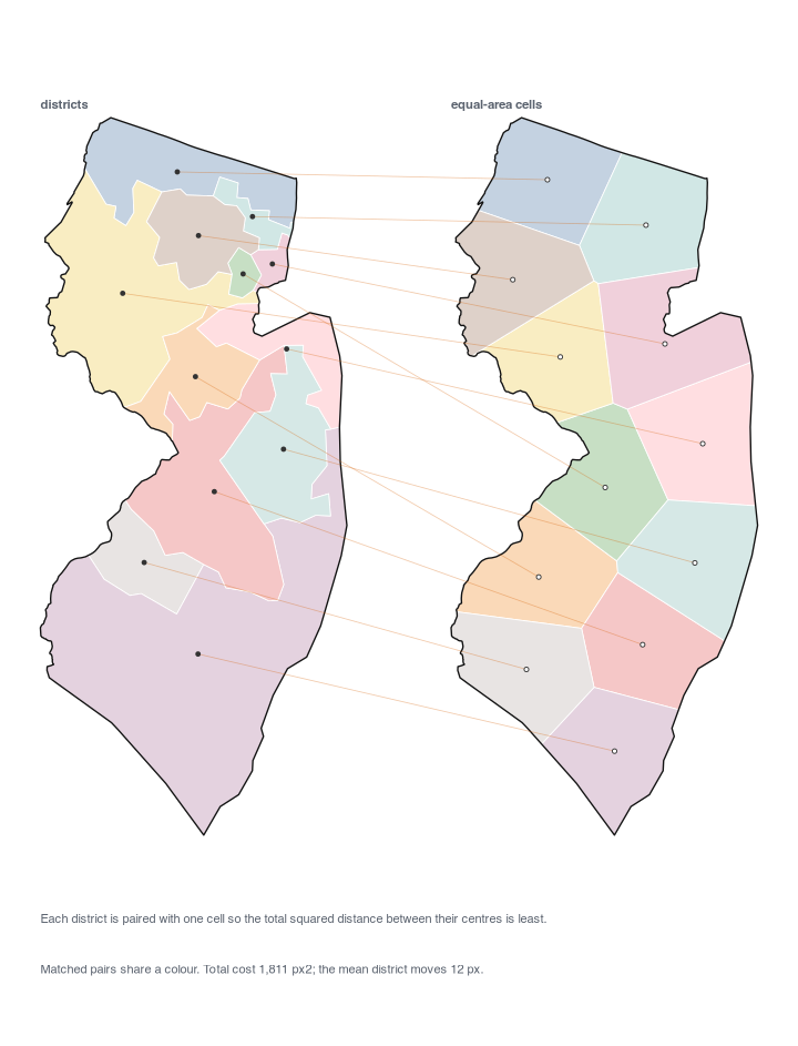
Matched pairs share a colour. The small dense districts in the north-east map to cells the same size as the large southern ones — which is the whole point of the cartogram, made visible.

The rule

Pair each district with exactly one cell so that the total squared distance between their centres is as small as possible.

That is a linear assignment problem. It is tempting to solve it greedily — take the closest pair, remove both, repeat — but greedy is not optimal and the failure is visible: one district gets stranded and has to cross the state to reach the last free cell. The optimum is found exactly by the Hungarian algorithm, in R/lib_assign.R.

For New Jersey the optimal total is about 1,810 px², and the mean district centre moves 12 px.

Why squared distance

Squaring penalises one long journey more than several short ones, so the optimum spreads the displacement around rather than accepting a single state- crossing move. It is also what the original notebook used, via munkres-js.

The implementation

hungarian(cost) is the O(n³) shortest-augmenting-path form (Jonker–Volgenant), with dual potentials and a virtual start column. About sixty lines of base R, no packages.

It self-tests on every build: test_hungarian() runs it against brute force on 40 random cost matrices and stops the build on any mismatch or invalid assignment. That check costs milliseconds and means a subtle indexing error in a hand-rolled solver cannot reach the output silently.

[assign] hungarian() matches brute force on 40 random cases

The matrix is small — at most 52×52, for California — so the solve is instantaneous. The whole 435-district assignment takes a few milliseconds.

Rectangular cases

The apportionment maps break the square assumption. A state that lost a seat has more cells than it has current districts, because cells are carved at max(seatsFrom, seatsTo). hungarian() handles a rectangular cost matrix directly when there are more columns than rows, and transposes when there are more rows than columns.

The cells left unmatched are exactly the seats that moved, which is how the apportionment map knows which cells to mark. Those carry no district id in the output, so nothing downstream can mistake them for real districts.

One consequence worth stating: for a comparison that does not end at the apportionment the boundary file was drawn under — 2000 → 2010 against 2022 lines — the districts correspond to neither endpoint, so no assignment is run at all and meta.districtsAttached is false.

What the output carries

Each district in the JSON gets both shapes and both anchors:

{
  "id": "NJ-01",
  "centroid": [x, y],   // its true geographic centre
  "target":   [x, y],   // the seed point of the cell it was matched to
  "geo":  { "type": "Polygon", ... },   // true geography
  "cell": { "type": "Polygon", ... }    // its equal-area counterpart
}

A renderer interpolates geo → cell and has everything it needs. Multipolygon parts are ordered largest-first so a morph library pairing an n-part shape with an m-part shape matches them sensibly.

Where the code lives

Back to placement, or carving cells.