Carving equal-area cells

Once placement has stopped moving the states, each one is subdivided into as many cells as it has seats — and the cells must come out roughly equal in area, because that is the entire point of the design. A district’s cell should carry the same visual weight whether it covers half of Montana or six blocks of Manhattan.

The figures come from R/41_method_figures.R, which re-runs the real subdivision for one state with the same functions and the same seed as the build. New Jersey is the worked example, for the same reason the original notebook used it: twelve districts in a small, awkward, non-convex shape.

The four steps

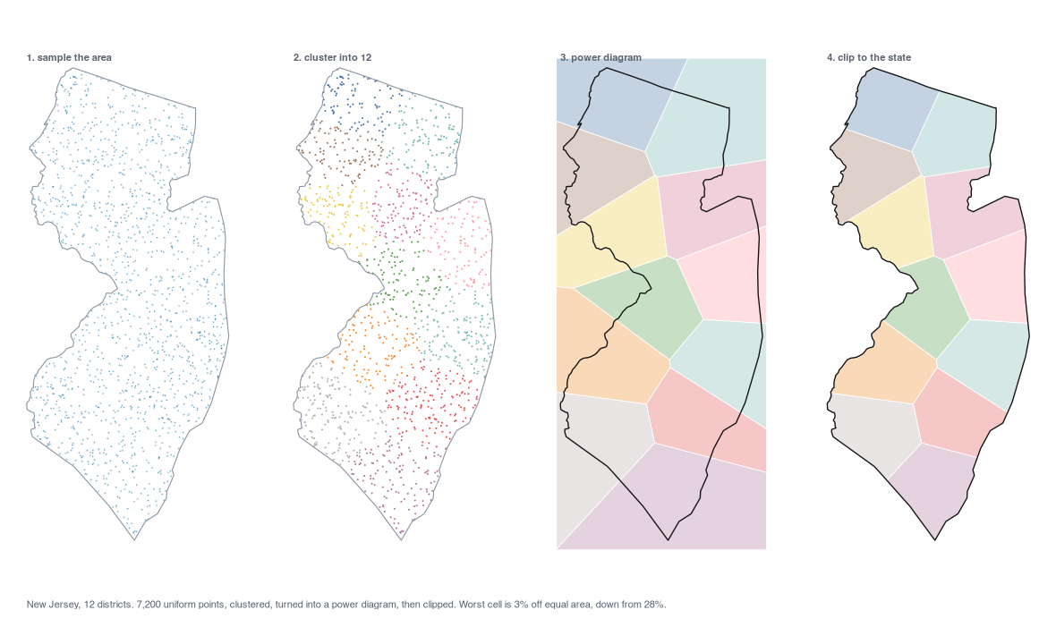
1. Sample the area. Scatter uniform random points across the state — 7,200 for New Jersey, 600 per seat with a floor and a ceiling. Points are allocated between a state’s parts in proportion to their area and placed by rejection sampling inside each part’s bounding box, so islands and peninsulas get their fair share. This is the only randomness in the pipeline, and it is seeded per state (SEED + i), so a rebuild reproduces the same cells exactly.

2. Cluster into as many groups as there are seats. k-means on a uniform point cloud is the trick: because the points are spread evenly over the area, clusters holding an equal number of points are clusters holding an equal amount of area. k-means minimises within-cluster variance, which also makes the groups compact rather than straggly.

3. Turn the clusters into polygons. The cells are the Voronoi diagram of the cluster centres — or rather a power diagram, which is the same construction with a per-site weight (see below). Both are built by intersecting half-planes one at a time, which is exact because the cells are convex and needs no topology library.

4. Clip to the state. The cells run past the border until mapshaper intersects them with the state outline. After that they tile it exactly, and the cell areas sum to the state’s area to within 0.25% — the remainder is sliver filtering.

Why plain k-means is not enough

k-means equalises variance, not area, and in an awkward shape those come apart badly.

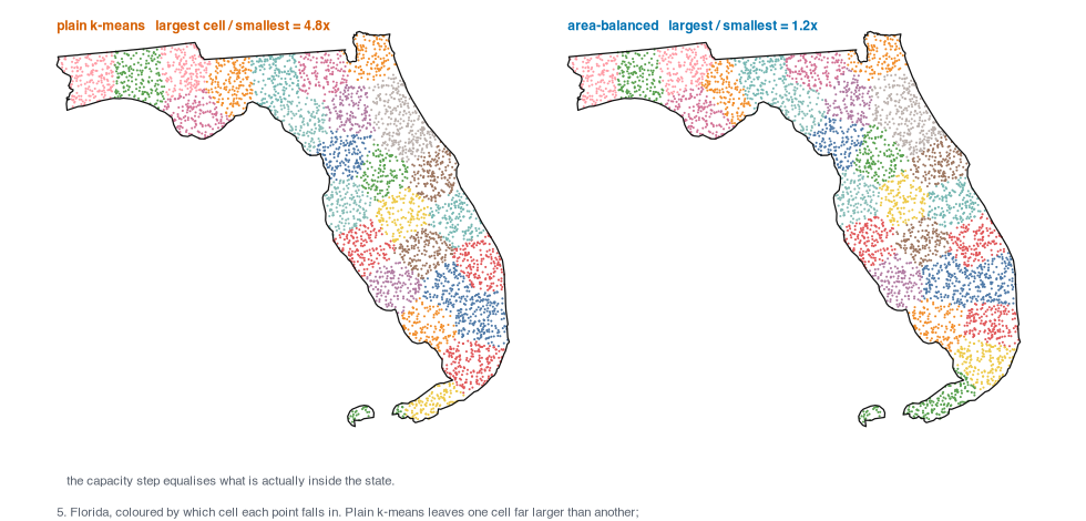
Florida is the case that forced the issue: a long panhandle joined to a long peninsula. Plain k-means leaves its largest cell 4.8× its smallest. After balancing that ratio is 1.15×.

(That 4.8× is measured on the point cloud, before mapshaper clips. On the finished clipped cells the same comparison runs 5.5× down to 1.24×.)

So balance_cells() alternates two moves until the areas even out:

• Lloyd step — move each site to the mean of the points it captured.
• Capacity step — raise the weight of an under-full cell, lower an over-full one. Weights turn the Voronoi diagram into a power diagram: the boundary between two sites is still a straight line, just shifted toward the lighter one.

Because the sample points all lie inside the state, the count a site captures is a Monte-Carlo estimate of its cell’s area after clipping — which is the area that actually matters. That is the part worth remembering: measuring the raw cell polygons instead reports ~17× for both methods and hides the whole effect, because most of a raw cell is the part that gets clipped away.

Across all 50 states, measured on the finished clipped cells, the worst within-state area ratio falls from 5.53 (Florida) to 1.24 (California), and the median from 1.38 to 1.11. Set BALANCE_ITERS=0 to build without it and reproduce the left-hand numbers.

Half-plane clipping

A Voronoi cell is the set of points closer to its site than to any other, so it is the intersection of one half-plane per rival site. Start with a rectangle covering the state and clip it, rival by rival, with Sutherland–Hodgman. The result is exact, convex by construction, and about forty lines of base R.

The power-diagram version is the same code with an offset: the bisector between sites i and j moves according to the difference of their weights.

(sj - si) · p  ≤  ( |sj|² - |si|² - wj + wi ) / 2

With wi = wj = 0 that is the ordinary perpendicular bisector, which is why one function serves both.

Cost

O(n²) half-plane clips per state, where n is the seat count — at most 52, for California. The expensive part is the point-in-polygon testing during sampling, which is why the sample size is capped. A full 50-state build takes about 20 seconds.

Where the code lives

Next: matching cells to districts.